Plotting#
tabensemb.trainer.Trainer provides some useful plotting methods to analyse the dataset or results.
[1]:
import torch
from tabensemb.trainer import Trainer
from tabensemb.model import *
from tabensemb.config import UserConfig
import tabensemb
import os
from tempfile import TemporaryDirectory

device = "cuda" if torch.cuda.is_available() else "cpu"
print("Using {} device".format(device))

temp_path = TemporaryDirectory()
tabensemb.setting["default_output_path"] = os.path.join(temp_path.name, "output")
tabensemb.setting["default_config_path"] = os.path.join(temp_path.name, "configs")
tabensemb.setting["default_data_path"] = os.path.join(temp_path.name, "data")

trainer = Trainer(device=device)
mpg_columns = [
    "mpg",
    "cylinders",
    "displacement",
    "horsepower",
    "weight",
    "acceleration",
    "model_year",
    "origin",
    "car_name",
]
cfg = UserConfig.from_uci("Auto MPG", column_names=mpg_columns, sep=r"\s+")
trainer.load_config(cfg)
trainer.load_data()
models = [
    PytorchTabular(trainer, model_subset=["Category Embedding"]),
    CatEmbed(trainer, model_subset=["Category Embedding"])
]
trainer.add_modelbases(models)
trainer.train(stderr_to_stdout=True)
Using cuda device
Downloading https://archive.ics.uci.edu/static/public/9/auto+mpg.zip to /tmp/tmp7ery7st7/data/Auto MPG.zip
cylinders is Integer and will be treated as a continuous feature.
model_year is Integer and will be treated as a continuous feature.
origin is Integer and will be treated as a continuous feature.
Unknown values are detected in ['horsepower']. They will be treated as np.nan.
The project will be saved to /tmp/tmp7ery7st7/output/auto-mpg/2023-10-08-13-00-16-0_UserInputConfig
Dataset size: 238 80 80
Data saved to /tmp/tmp7ery7st7/output/auto-mpg/2023-10-08-13-00-16-0_UserInputConfig (data.csv and tabular_data.csv).

-------------Run PytorchTabular-------------

Training Category Embedding
Global seed set to 42
2023-10-08 13:00:17,416 - {pytorch_tabular.tabular_model:473} - INFO - Preparing the DataLoaders
2023-10-08 13:00:17,417 - {pytorch_tabular.tabular_datamodule:290} - INFO - Setting up the datamodule for regression task
2023-10-08 13:00:17,424 - {pytorch_tabular.tabular_model:521} - INFO - Preparing the Model: CategoryEmbeddingModel
2023-10-08 13:00:17,434 - {pytorch_tabular.tabular_model:268} - INFO - Preparing the Trainer
/home/xlluo/anaconda3/envs/tabular_ensemble/lib/python3.10/site-packages/pytorch_lightning/trainer/connectors/accelerator_connector.py:589: LightningDeprecationWarning: The Trainer argument `auto_select_gpus` has been deprecated in v1.9.0 and will be removed in v2.0.0. Please use the function `pytorch_lightning.accelerators.find_usable_cuda_devices` instead.
  rank_zero_deprecation(
Auto select gpus: [0]
GPU available: True (cuda), used: True
TPU available: False, using: 0 TPU cores
IPU available: False, using: 0 IPUs
HPU available: False, using: 0 HPUs
2023-10-08 13:00:18,152 - {pytorch_tabular.tabular_model:582} - INFO - Training Started
You are using a CUDA device ('NVIDIA GeForce RTX 3090') that has Tensor Cores. To properly utilize them, you should set `torch.set_float32_matmul_precision('medium' | 'high')` which will trade-off precision for performance. For more details, read https://pytorch.org/docs/stable/generated/torch.set_float32_matmul_precision.html#torch.set_float32_matmul_precision
LOCAL_RANK: 0 - CUDA_VISIBLE_DEVICES: [0]

  | Name             | Type                      | Params
---------------------------------------------------------------
0 | _backbone        | CategoryEmbeddingBackbone | 11.4 K
1 | _embedding_layer | Embedding1dLayer          | 14
2 | head             | LinearHead                | 33
3 | loss             | MSELoss                   | 0
---------------------------------------------------------------
11.4 K    Trainable params
0         Non-trainable params
11.4 K    Total params
0.046     Total estimated model params size (MB)
Epoch: 1/300, Train loss: 677.8015, Val loss: 582.9557, Min val loss: 582.9557, Epoch time: 0.010s.
Epoch: 20/300, Train loss: 353.7851, Val loss: 302.0203, Min val loss: 302.0203, Epoch time: 0.007s.
Epoch: 40/300, Train loss: 85.0776, Val loss: 62.1153, Min val loss: 62.1153, Epoch time: 0.007s.
Epoch: 60/300, Train loss: 45.2654, Val loss: 34.2778, Min val loss: 34.2691, Epoch time: 0.007s.
Epoch: 80/300, Train loss: 33.9537, Val loss: 26.8622, Min val loss: 26.8622, Epoch time: 0.007s.
Epoch: 100/300, Train loss: 26.9038, Val loss: 23.2417, Min val loss: 23.2372, Epoch time: 0.007s.
Epoch: 120/300, Train loss: 24.9622, Val loss: 20.4360, Min val loss: 20.4360, Epoch time: 0.007s.
Epoch: 140/300, Train loss: 24.1636, Val loss: 19.4010, Min val loss: 19.4010, Epoch time: 0.007s.
Epoch: 160/300, Train loss: 22.9200, Val loss: 18.0232, Min val loss: 17.9749, Epoch time: 0.007s.
Epoch: 180/300, Train loss: 19.7677, Val loss: 16.9469, Min val loss: 16.9469, Epoch time: 0.007s.
Epoch: 200/300, Train loss: 17.9390, Val loss: 16.6545, Min val loss: 16.4093, Epoch time: 0.007s.
Epoch: 220/300, Train loss: 19.4496, Val loss: 15.4451, Min val loss: 15.1788, Epoch time: 0.007s.
Epoch: 240/300, Train loss: 16.0483, Val loss: 14.5508, Min val loss: 14.5508, Epoch time: 0.008s.
Epoch: 260/300, Train loss: 16.4672, Val loss: 13.8354, Min val loss: 13.8354, Epoch time: 0.007s.
Epoch: 280/300, Train loss: 13.6031, Val loss: 12.9315, Min val loss: 12.9315, Epoch time: 0.007s.
Epoch: 300/300, Train loss: 16.5369, Val loss: 12.3673, Min val loss: 12.3673, Epoch time: 0.007s.
`Trainer.fit` stopped: `max_epochs=300` reached.
2023-10-08 13:00:21,684 - {pytorch_tabular.tabular_model:584} - INFO - Training the model completed
2023-10-08 13:00:21,684 - {pytorch_tabular.tabular_model:1258} - INFO - Loading the best model
/home/xlluo/anaconda3/envs/tabular_ensemble/lib/python3.10/site-packages/pytorch_lightning/utilities/cloud_io.py:33: LightningDeprecationWarning: `pytorch_lightning.utilities.cloud_io.get_filesystem` has been deprecated in v1.8.0 and will be removed in v2.0.0. Please use `lightning_fabric.utilities.cloud_io.get_filesystem` instead.
  rank_zero_deprecation(
Training mse loss: 11.25175
Validation mse loss: 12.36725
Testing mse loss: 7.83801
Trainer saved. To load the trainer, run trainer = load_trainer(path='/tmp/tmp7ery7st7/output/auto-mpg/2023-10-08-13-00-16-0_UserInputConfig/trainer.pkl')

-------------PytorchTabular End-------------


-------------Run CatEmbed-------------

Training Category Embedding
GPU available: True (cuda), used: True
TPU available: False, using: 0 TPU cores
IPU available: False, using: 0 IPUs
HPU available: False, using: 0 HPUs
You are using a CUDA device ('NVIDIA GeForce RTX 3090') that has Tensor Cores. To properly utilize them, you should set `torch.set_float32_matmul_precision('medium' | 'high')` which will trade-off precision for performance. For more details, read https://pytorch.org/docs/stable/generated/torch.set_float32_matmul_precision.html#torch.set_float32_matmul_precision
LOCAL_RANK: 0 - CUDA_VISIBLE_DEVICES: [0]

  | Name                | Type        | Params
----------------------------------------------------
0 | default_loss_fn     | MSELoss     | 0
1 | default_output_norm | Identity    | 0
2 | linear              | Sequential  | 11.4 K
3 | embed               | Embedding1d | 14
4 | head                | Linear      | 33
----------------------------------------------------
11.4 K    Trainable params
9         Non-trainable params
11.4 K    Total params
0.046     Total estimated model params size (MB)
Epoch: 1/300, Train loss: 677.8015, Val loss: 583.1656, Min val loss: 583.1656, Min ES val loss: 583.1656, Epoch time: 0.006s.
Epoch: 20/300, Train loss: 353.7850, Val loss: 301.6606, Min val loss: 301.6606, Min ES val loss: 301.6606, Epoch time: 0.005s.
Epoch: 40/300, Train loss: 85.0776, Val loss: 62.0647, Min val loss: 62.0647, Min ES val loss: 62.0647, Epoch time: 0.005s.
Epoch: 60/300, Train loss: 45.2654, Val loss: 34.2774, Min val loss: 34.2689, Min ES val loss: 34.2689, Epoch time: 0.005s.
Epoch: 80/300, Train loss: 33.9537, Val loss: 26.8621, Min val loss: 26.8621, Min ES val loss: 26.8621, Epoch time: 0.005s.
Epoch: 100/300, Train loss: 26.9038, Val loss: 23.2417, Min val loss: 23.2372, Min ES val loss: 23.2372, Epoch time: 0.005s.
Epoch: 120/300, Train loss: 24.9622, Val loss: 20.4360, Min val loss: 20.4360, Min ES val loss: 20.4360, Epoch time: 0.005s.
Epoch: 140/300, Train loss: 24.1636, Val loss: 19.4010, Min val loss: 19.4010, Min ES val loss: 19.4010, Epoch time: 0.005s.
Epoch: 160/300, Train loss: 22.9200, Val loss: 18.0232, Min val loss: 17.9749, Min ES val loss: 17.9749, Epoch time: 0.005s.
Epoch: 180/300, Train loss: 19.7677, Val loss: 16.9469, Min val loss: 16.9469, Min ES val loss: 16.9469, Epoch time: 0.005s.
Epoch: 200/300, Train loss: 17.9390, Val loss: 16.6545, Min val loss: 16.4093, Min ES val loss: 16.4093, Epoch time: 0.005s.
Epoch: 220/300, Train loss: 19.4496, Val loss: 15.4451, Min val loss: 15.1788, Min ES val loss: 15.1788, Epoch time: 0.005s.
Epoch: 240/300, Train loss: 16.0483, Val loss: 14.5508, Min val loss: 14.5508, Min ES val loss: 14.5508, Epoch time: 0.005s.
Epoch: 260/300, Train loss: 16.4672, Val loss: 13.8354, Min val loss: 13.8354, Min ES val loss: 13.8354, Epoch time: 0.005s.
Epoch: 280/300, Train loss: 13.6031, Val loss: 12.9315, Min val loss: 12.9315, Min ES val loss: 12.9315, Epoch time: 0.005s.
Epoch: 300/300, Train loss: 16.5369, Val loss: 12.3673, Min val loss: 12.3673, Min ES val loss: 12.3673, Epoch time: 0.005s.
`Trainer.fit` stopped: `max_epochs=300` reached.
Training mse loss: 11.25176
Validation mse loss: 12.36726
Testing mse loss: 7.83801
Trainer saved. To load the trainer, run trainer = load_trainer(path='/tmp/tmp7ery7st7/output/auto-mpg/2023-10-08-13-00-16-0_UserInputConfig/trainer.pkl')

-------------CatEmbed End-------------
If LaTeX is detected, matplotlib.rc("text", usetex=True) is called to use LaTeX for a better text appearance. However, if there exist "_" in feature names, LaTeX will throw errors. Here we reset defaults of matplotlib.rcParams to disable LaTeX.
[2]:
import matplotlib
import matplotlib.pyplot as plt
matplotlib.rcParams.update(matplotlib.rcParamsDefault)
plt.rcParams["figure.autolayout"] = True
Trainer.plot_fill_rating will show a histogram of the filling ratio of data points. There are several data points with missing entries.
Remark: All methods introduced in this part pass arguments, such as figure_kwargs, bar_kwargs, pairplot_kwargs, etc., to corresponding functions for limited but sufficient customization. See the API docs for their meanings.
Remark: Colors can be globally controlled by replacing tabensemb.utils.global_palette. For some methods, clr can be given to control colors. One can also pass kwargs to arguments like bar_kwargs to over-ride default behaviors including colors.
Remark: The argument category is used to distinguish different data points in the plot. The argument is available for many of the methods introduced in this part.
[3]:
trainer.plot_fill_rating(figure_kwargs=dict(figsize=(4,3), dpi=150), category="origin")

[3]:
<Axes: xlabel='Fill rating', ylabel='Density'>
Trainer.plot_presence_ratio will show the filling ratio of features. There are missing entries only in the horsepower feature.
[4]:
trainer.plot_presence_ratio()

[4]:
<Axes: xlabel='Data presence ratio'>
Trainer.plot_feature_box will show the box plot of features.
[5]:
trainer.plot_feature_box(imputed=True, figure_kwargs=dict(figsize=(4, 4)))

[5]:
<Axes: xlabel='Values (Scaled)'>
Trainer.plot_pairplot will show correlations between each two features. It uses seaborn.pairplot to achieve this, so the plot can be customized by passing the pairplot_kwargs argument. See the documentation for possible arguments.
[6]:
trainer.plot_pairplot(pairplot_kwargs=dict(height=1))
/home/xlluo/anaconda3/envs/tabular_ensemble/lib/python3.10/site-packages/seaborn/axisgrid.py:118: UserWarning: The figure layout has changed to tight
  self._figure.tight_layout(*args, **kwargs)
/home/xlluo/hdd/tabular_ensemble/tabensemb/trainer/trainer.py:3848: UserWarning: The figure layout has changed to tight
  plt.tight_layout()

[6]:
<seaborn.axisgrid.PairGrid at 0x7f61ac713820>
Trainer.plot_corr will show the correlation coefficients between each two features. It uses the Pearson correlation by default.
[7]:
trainer.plot_corr(imputed=True, figure_kwargs=dict(figsize=(5, 5)), imshow_kwargs=dict(cmap="RdBu"))

[7]:
<Axes: >
Trainer.plot_corr_with_label focuses on the correlation between the target and each feature.
[8]:
trainer.plot_corr_with_label(imputed=True, figure_kwargs={"figsize": (6, 5)}, order="descending")

[8]:
<Axes: xlabel='Correlation with mpg'>
Trainer.plot_pca_2d_visual will show a scatter plot where the x and y axes are the first and second principal components from PCA, respectively.
[9]:
trainer.plot_pca_2d_visual(features=trainer.cont_feature_names)

[9]:
<Axes: xlabel='1st principal component', ylabel='2nd principal component'>
Trainer.plot_scatter offers the utility to plot one feature against another. Here is an example that plots scatters between weight and horsepower whose model_year is in the range \([70, 74]\).
Remark: select_by_value_kwargs is the argument of DataModule.select_by_value which returns indices of datapoints that have specified values in the specified columns.
[10]:
trainer.plot_scatter(x_col="weight", y_col="horsepower", scatter_kwargs={"color": "#635380", "s": 15, "marker": "s"}, select_by_value_kwargs={"selection": {"model_year": (70, 74)}}, kde_color=True)

[10]:
<Axes: xlabel='weight', ylabel='horsepower'>
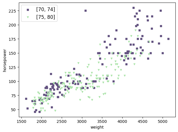
Trainer.plot_on_one_axes can plot multiple items (like scatters) on one matplotlib.axes.Axes instance. Here is an example that calls Trainer.plot_scatter twice to plots a group of scatters whose model_year is in the range \([70, 74]\) and the other group of scatters whose model_year is in the range \([75, 80]\).
Remark: Most methods in this part have the argument ax which should be a matplotlib.axes.Axes instance. If it is given, no new figure will be created and the item will be plotted on the ax directly. This is how we implement Trainer.plot_on_one_axes.
[11]:
trainer.plot_on_one_axes(
    meth_name="plot_scatter",
    meth_kwargs_ls=[
        dict(scatter_kwargs={"color": "#635380", "s": 15, "marker": "s", "label": "[70, 74]"}, select_by_value_kwargs={"selection": {"model_year": (70, 74)}}),
        dict(scatter_kwargs={"color": "#ACE4AA", "s": 15, "marker": "v", "label": "[75, 80]"}, select_by_value_kwargs={"selection": {"model_year": (75, 80)}})
    ],
    meth_fix_kwargs=dict(
        x_col="weight",
        y_col="horsepower",
        imputed=False,
    ),
    xlabel="weight",
    ylabel="horsepower",
    legend=True,
)
[11]:
<Axes: xlabel='weight', ylabel='horsepower'>
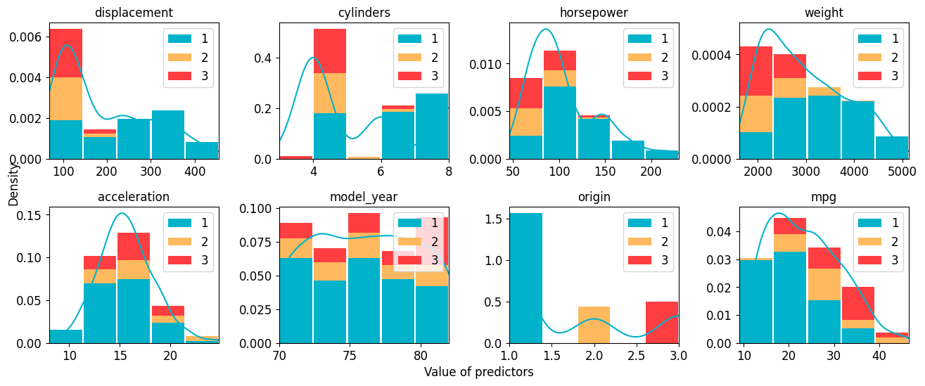
Trainer.plot_hist_all shows the histogram for each feature. If the argument category is given, histograms of each unique value of the category column will be plotted separately and stacked together.
Remark: All methods with the postfix _all introduced in this part utilize corresponding methods without the postfix. For example, Trainer.plot_hist_all calls Trainer.plot_hist for multiple times.
[12]:
_ = trainer.plot_hist_all(imputed=False, kde=True, hist_kwargs={"bins": 5}, category="origin", legend_kwargs={"loc": "upper right"})
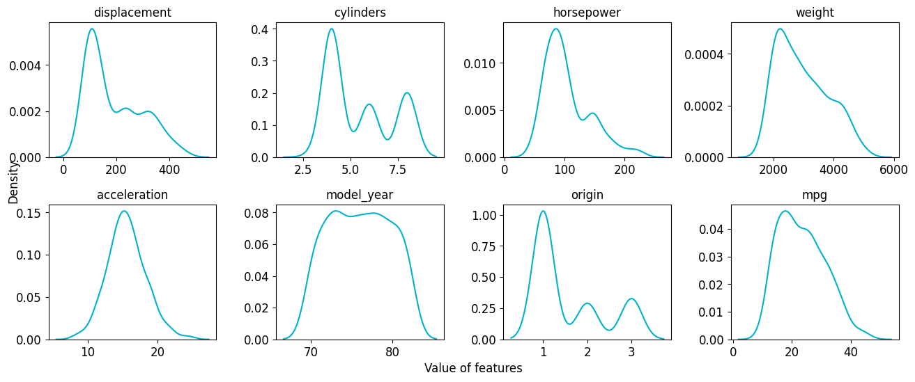
Trainer.plot_kde_all shows 1d KDE results for each feature.
[13]:
_ = trainer.plot_kde_all(imputed=False)
Trainer.plot_kde can also plot bi-variate gaussian kernel density.
[14]:
trainer.plot_kde(x_col="displacement", y_col="cylinders", kdeplot_kwargs=dict(fill=True, thresh=0, levels=100))

[14]:
<Axes: xlabel='displacement', ylabel='cylinders'>
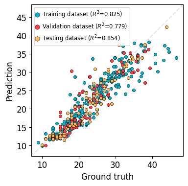
Trainer.plot_truth_pred will show the comparison between ground truth values and predictions.
[15]:
trainer.plot_truth_pred(program="PytorchTabular", model_name="Category Embedding", log_trans=False, legend_kwargs=dict(fontsize="x-small"), figure_kwargs=dict(figsize=(4, 4)))
Training MSE Loss: 11.2517, R2: 0.8254
Validation MSE Loss: 12.3672, R2: 0.7791
Testing MSE Loss: 7.8380, R2: 0.8542
[15]:
<Axes: xlabel='Ground truth', ylabel='Prediction'>
Trainer.plot_loss shows the curves of training loss and/or validation loss. It is supported for PytorchTabular, WideDeep or any TorchModel-based models.
[16]:
trainer.plot_loss(program="PytorchTabular", model_name="Category Embedding", train_val="both", restored_epoch_mark_if_last=True)
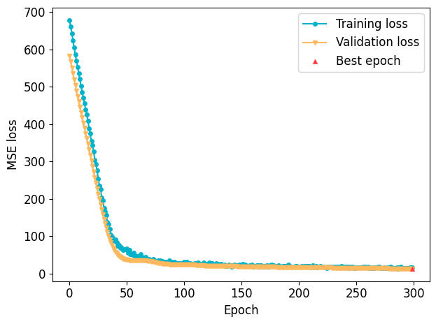
[16]:
<Axes: xlabel='Epoch', ylabel='MSE loss'>
Trainer.plot_feature_importance calculates and plots feature importance. Two methods are supported to calculate feature importance: permutation and shap. Permutation feature importance is the decrease of the metric when permuting (shuffling) the feature. SHAP is a game theory approach.
They might get different results.
For pytorch based models, we use captum (link) and shap.DeepExplainer (link) for faster calculations.
[17]:
trainer.plot_feature_importance(program="PytorchTabular", model_name="Category Embedding", figure_kwargs=dict(figsize=(5, 4)))
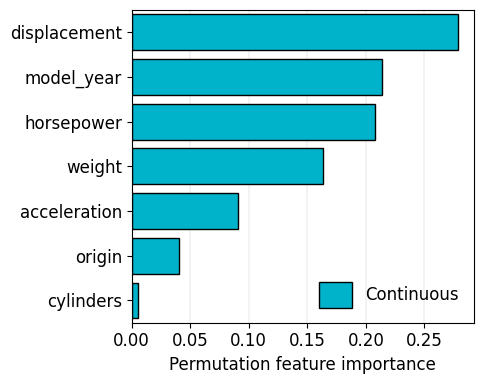
[17]:
<Axes: xlabel='Permutation feature importance'>
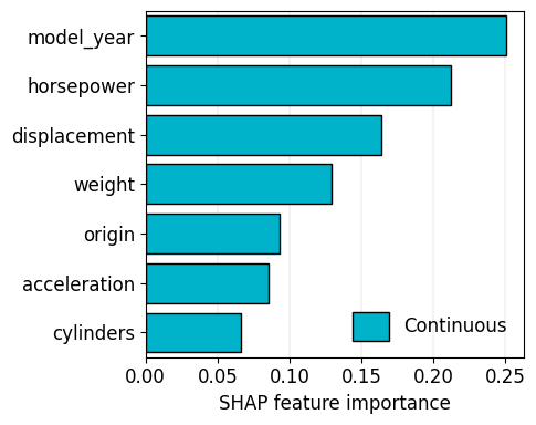
[18]:
import warnings

with warnings.catch_warnings():
    warnings.filterwarnings("ignore")
    trainer.plot_feature_importance(program="CatEmbed", model_name="Category Embedding", method="shap", figure_kwargs=dict(figsize=(5, 4)))
Feature importance less than 1e-5: ['Unscaled-0', 'Unscaled-1', 'Unscaled-2', 'Unscaled-3', 'Unscaled-4', 'Unscaled-5', 'Unscaled-6']
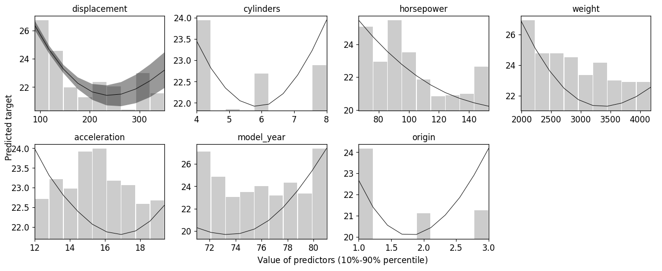
Trainer.plot_partial_dependence_all uses bootstrap sampling to resample the dataset, fits the model on the resampled dataset, and obtains sequential predictions when assigning sequential values to a feature, to see the dependency of predictions on a feature.
[19]:
with warnings.catch_warnings():
    warnings.filterwarnings("ignore")
    trainer.plot_partial_dependence_all(program="PytorchTabular", model_name="Category Embedding", n_bootstrap=3, grid_size=10, log_trans=False, upper_lim=9, lower_lim=2, CI=0.95)
Calculate PDP:  displacement
Calculate PDP:  cylinders
Calculate PDP:  horsepower
Calculate PDP:  weight
Calculate PDP:  acceleration
Calculate PDP:  model_year
Calculate PDP:  origin
Trainer.plot_err_hist shows the distribution of errors. If the argument category is given, one can try to analyse the relationship between categories and errors.
[20]:
trainer.plot_err_hist(program="PytorchTabular", model_name="Category Embedding", metric="mse", category="origin", legend_kwargs={"title": "origin"})
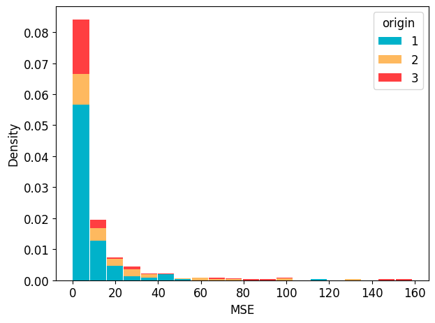
[20]:
<Axes: xlabel='MSE', ylabel='Density'>
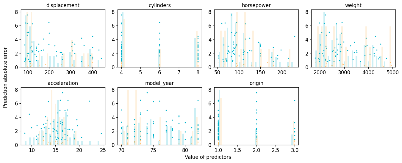
Trainer.plot_partial_err_all shows the distribution of absolute error with respect to feature values. If the density of high error predictions is high in a certain range of a certain feature, data augmentation or additional experiments might be required.
[21]:
_ = trainer.plot_partial_err_all(program="PytorchTabular", model_name="Category Embedding")